What this post is about

There’s quite the fuzz about ‘objective’ measures of technology use. When we study the effects of tech use on well-being, we often just ask people to report how much they used tech. Turns out, people aren’t really good at estimating their tech use. When we compare their subjective estimates to logged tech use (hence ‘objective’), the correlation between the two is rather low as this meta-analysis reports.

Several researchers are interested in what predicts that low accuracy. One hypothesis that has been brought forward repeatedly (e.g., here) is that heavy users will mis-estimate their use more. In operational terms: the higher your objective use, the larger the discrepancy between your estimated use and objective use. Most of the time, discrepancy is defined as absolute difference between objective and subjective tech use (abs(objetice-subjective)). Then, we correlate that discrepancy with objective use to find out whether those who use tech more are also less accurate in their estimates.

That got me thinking. Isn’t it weird to predict something with parts of itself? What I mean is: Discrepancy is a transformation of objective and subjective use, so you’d expect that that transformation is related to one of its components. (At least that’s my intuition. Not like I’d have math skills to back that intuition up formally.)

So I wanted to know what happens if you correlate discrepancy between objective and subjective use with objective use if both subjective and objective are completely unrelated. If my intuition is wrong, you’d expect that discrepancy is also unrelated to objective use. In other words, I wanted to see what effect the calculation of discrepancy has on Type I error (and effect size).

Simulation

Below a quick-n-dirty simulation: 10,000 times I simulated uncorrelated objective (actual) and subjective (estimated) use in a sample size that’s fairly typical of papers that compare objective and subjective use. In the simulation, I don’t estimate a normal distribution for phone use in minutes, simply because we know that minutes on your phone a) cannot be negative, b) are likely right-skewed. For that reason, I chose a Gamma distribution.

The exact values don’t matter, but I simulated within a minute range that seems like a reasonable amount of time on your phone for a day and is in line with the literature. I also took into account that this meta-analysis found that subjective phone use is usually an overestimate compared to actual, objective phone use. The distributions look like below and are fairly representative of how distributions look like in the literature. Note that nobody has a zero, the distribution just makes it look like that. But there are several low values.

library(tidyverse)
set.seed(42)

estimated <- 
  tibble(
    minutes = rgamma(1000, 3, 0.03)
  )

actual <- 
  tibble(
    minutes = rgamma(1000, 2.8, 0.032)
  )

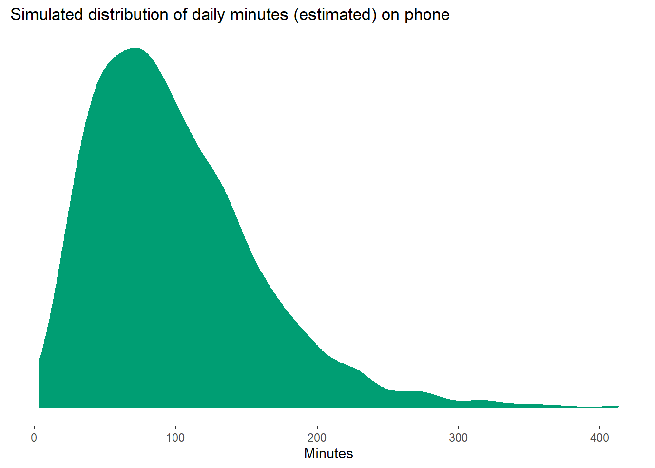
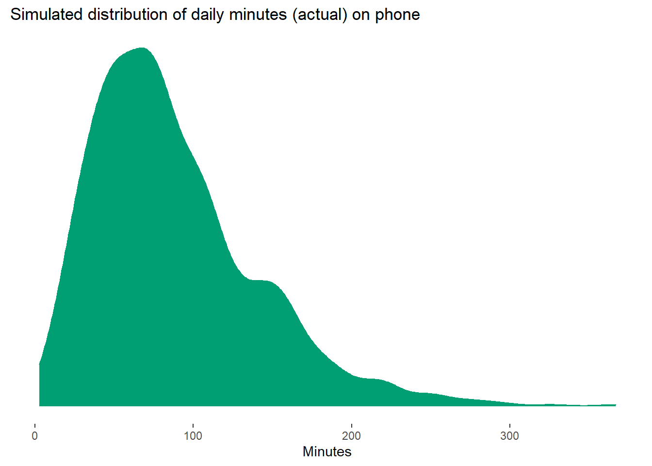
The mean of the estimated minutes is 99.57; mean of actual minutes is 87.93; the discrepancy between those two means is 11.64.

So for each of the 10,000 distributions, I calculate discrepancy as the absolute difference and obtain:

• correlation and p-value between objective and subjective use
• correlation and p-value between objective use and discrepancy

I ignored that the distribution of the variable isn’t normal for now. (Yes, I know loops in R are iffy, but I find them easier than map. Please let me know a better way to do this, always happy to get tips on code.)

# empty tibble where we'll store results in the loop below
results <- tibble(
  iteration = c(),
  raw_cor = c(),
  raw_p = c(),
  dis_cor = c(),
  dis_p = c()
)

# sample size in paper
N <- 300

for (run in 1:1e4){
  dat <- # data set for this run
    tibble(
      pp = 1:N, # participant
      estimated = rgamma(N, 3, 0.03), # estimated use
      actual = rgamma(N, 2.8, 0.032), # actual use
      discrepancy = abs(actual - estimated) # their absolute difference
    )
  
  raw_correlation <- with(dat, cor.test(actual, estimated)) # correlation between (unrelated) actual and estimated use
  
  discrepancy_correlation <- with(dat, cor.test(actual, discrepancy)) # correlation between absolute difference and actual use
  
  run_results <- # store the results from the two correlations of this run
    tibble(
      iteration = run,
      raw_cor = raw_correlation$estimate,
      raw_p = raw_correlation$p.value,
      dis_cor = discrepancy_correlation$estimate,
      dis_p = discrepancy_correlation$p.value
    )
  
  results <- # store results of this run in overall results
    bind_rows(
      results,
      run_results
    )
}

Results

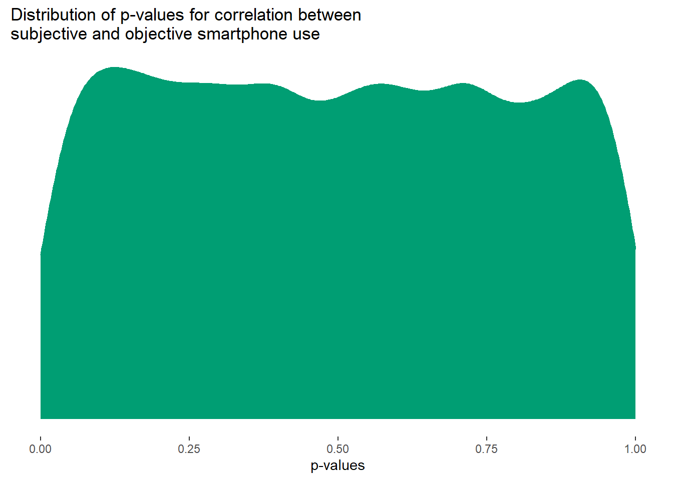
As expected, mean(results$raw_p < .05) = 4.84% of correlations between objective and subjective use are significant, pretty close to our nominal (and expected) Type I error rate. The p-values are distributed uniformly, as expected with a null effect.

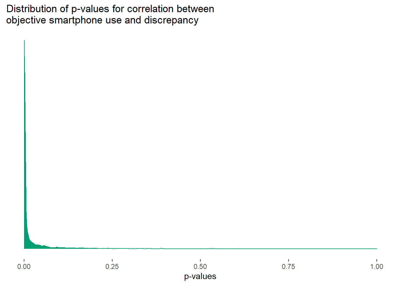
But for the correlation between discrepancy and objective use, the Type I error rate is extremely high, mean(results$dis_p < .05) ~ 83.39%, with many low p-values.

Also, the mean effect sizes for the raw correlation are close to zero, as simulated, (r = -0.00130), but large for the discrepancy correlation (r = 0.20).

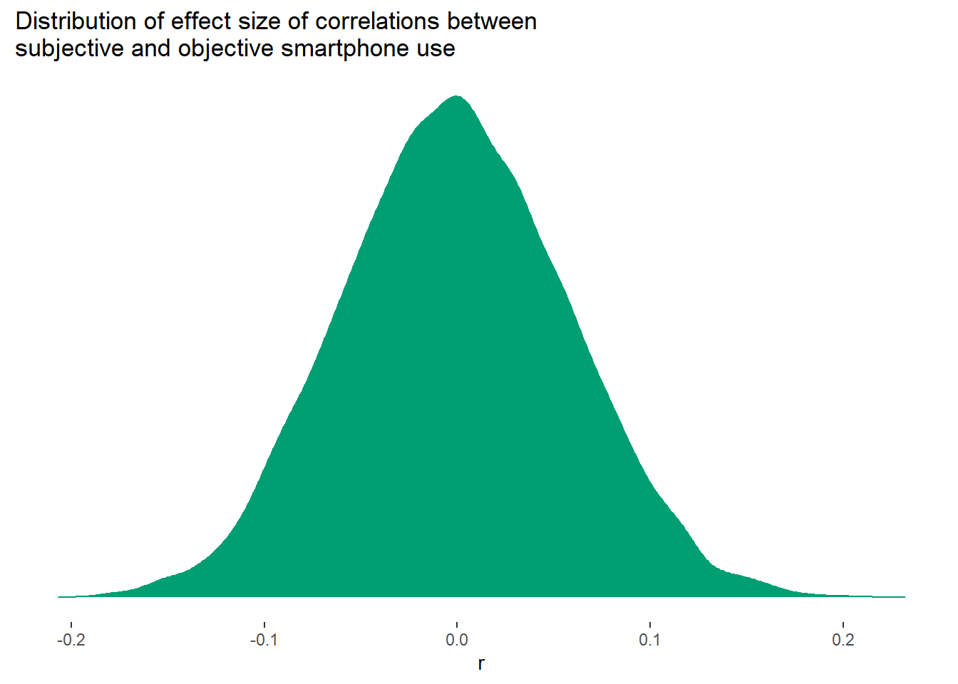
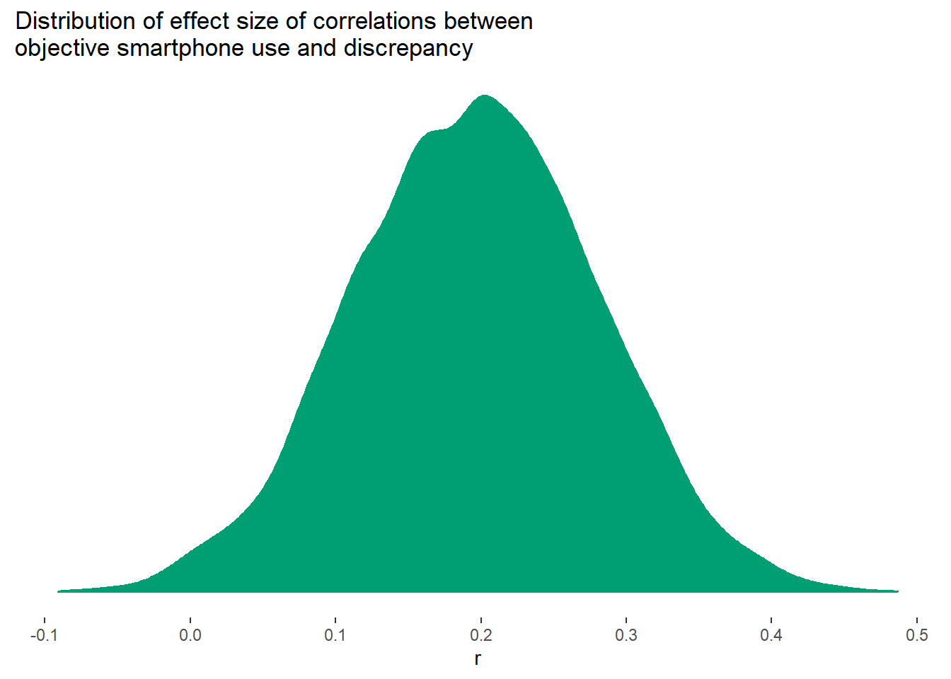
The raw correlations have a lower SD (0.06) than the discrepany correlations (0.08).

So what does this mean?

I’m not really sure. It might be as simple as saying: predicting something with one of its components will necessarily lead to some strange results. So positive correlations between objective use and discrepancy might be severely inflated or even entirely false positives. In other words, heavy users might not be less accurate.

Then again, it’s entirely possible that there’s some math magic here that I don’t see. As you can tell, I’m still not sure what to think about this. But I thought I’d share and get some feedback. So please let me know what you think.